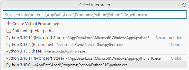
** vscode에서 파이썬 제대로 못잡을 때,
1. ctrl + shift + p
2. python: Select interpreter
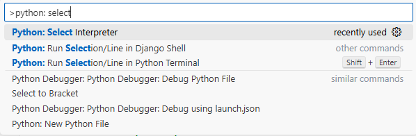
3. 사용할 파이썬 선택
1. Simplified hypothesis
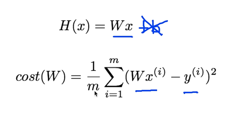
simplified 모델은 위와 같고, 결국에는 cost functino을 최소화 하는 W를 구하는게 목표이다.
import os
os.environ['TF_CPP_MIN_LOG_LEVEL'] = '1'
import tensorflow.compat.v1 as tf
tf.disable_v2_behavior()
import matplotlib.pyplot as plt

X = [1, 2, 3]
Y = [1, 2, 3]

W = tf.placeholder(tf.float32)

# Our hypothesis for linear model X * W
hypothesis = X * W

# cost/loss function
cost = tf.reduce_mean(tf.square(hypothesis - Y))

# Variables for plotting cost function
W_history = []
cost_history = []

# Launch the graph in a session.
with tf.Session() as sess:
    for i in range(-30, 50):
        curr_W = i * 0.1
        curr_cost = sess.run(cost, feed_dict={W: curr_W})

        W_history.append(curr_W)
        cost_history.append(curr_cost)

# Show the cost function
plt.plot(W_history, cost_history)
plt.show()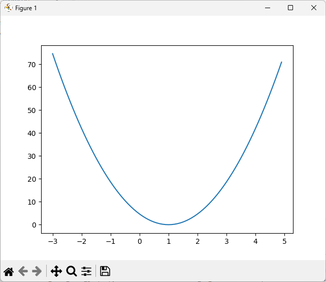
cost 함수는 위와 같다. cost를 최적화 하는 값은 대략 1임을 알 수 있다.
2. Gradient descent
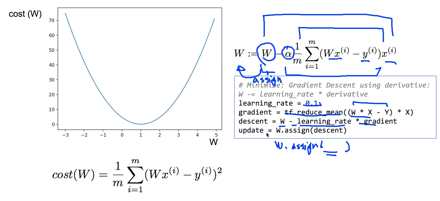
1. learning_rate는 상수로 0.1로 잡는다.
2. gradient는 (W*X - Y) * X를 평균 낸 tf.reduce_mean((W*X - Y) * X) 이다.
3. update = W.assign(descent) -> 계산된 descent 값을 W에 **덮어쓰기(assign)**하는 연산 객체 update를 그리면 된다.
import os
os.environ['TF_CPP_MIN_LOG_LEVEL'] = '1'
import tensorflow.compat.v1 as tf
tf.disable_v2_behavior()

x_data = [1, 2, 3]
y_data = [1, 2, 3]

# Try to find values for W and b to compute y_data = W * x_data
# We know that W should be 1
# But let's use TensorFlow to figure it out
W = tf.Variable(tf.random_normal([1]), name="weight")

X = tf.placeholder(tf.float32)
Y = tf.placeholder(tf.float32)

# Our hypothesis for linear model X * W
hypothesis = X * W

# cost/loss function
cost = tf.reduce_mean(tf.square(hypothesis - Y))

# Minimize: Gradient Descent using derivative: W -= learning_rate * derivative
learning_rate = 0.1
gradient = tf.reduce_mean((W * X - Y) * X)
descent = W - learning_rate * gradient
update = W.assign(descent)

# Launch the graph in a session.
with tf.Session() as sess:
    # Initializes global variables in the graph.
    sess.run(tf.global_variables_initializer())

    for step in range(21):
        _, cost_val, W_val = sess.run(
            [update, cost, W], feed_dict={X: x_data, Y: y_data}
        )
        print(step, cost_val, W_val)
# step cost W
0 1.7758361 [0.6709993]
1 0.50512683 [0.824533]
2 0.14368047 [0.9064176]
3 0.0408691 [0.9500894]
4 0.011624992 [0.97338104]
5 0.003306655 [0.98580325]
6 0.0009405531 [0.99242836]
7 0.0002675377 [0.9959618]
8 7.6099204e-05 [0.99784625]
9 2.1646554e-05 [0.9988513]
10 6.157729e-06 [0.9993874]
11 1.7512493e-06 [0.99967325]
12 4.9832533e-07 [0.9998257]
13 1.4174957e-07 [0.9999071]
14 4.028467e-08 [0.9999504]
15 1.1476611e-08 [0.99997354]
16 3.268383e-09 [0.9999859]
17 9.329296e-10 [0.9999925]
18 2.6142763e-10 [0.999996]
19 7.3949735e-11 [0.99999785]
20 2.1486812e-11 [0.99999887]결과로 cost값이 계속 작아질 때 W값이 1에 수렴함을 볼 수 있다.
2. Gradient descent, using GradientDescentOptimizer for tensorflow
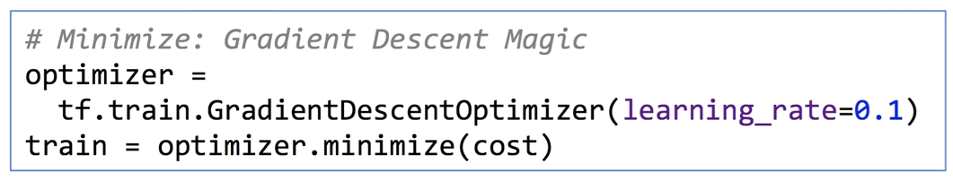
위와 같이 미분값이 쉬울 때는 직접 대입할 수 있지만 tensorflow에서 GradientDescentOptimizer를 제공하고 optimizer에 minimize 메소드를 통해 cost가 최소가 되게 구할 수 있다.
import os
os.environ['TF_CPP_MIN_LOG_LEVEL'] = '1'
import tensorflow.compat.v1 as tf
tf.disable_v2_behavior()

# tf Graph Input
X = [1, 2, 3]
Y = [1, 2, 3]

# Set wrong model weights
W = tf.Variable(5.0)

# Linear model
hypothesis = X * W

# cost/loss function
cost = tf.reduce_mean(tf.square(hypothesis - Y))

# Minimize: Gradient Descent Optimizer
train = tf.train.GradientDescentOptimizer(learning_rate=0.1).minimize(cost)

# Launch the graph in a session.
with tf.Session() as sess:
    # Initializes global variables in the graph.
    sess.run(tf.global_variables_initializer())

    for step in range(101):
        _, W_val = sess.run([train, W])
        print(step, W_val)
0 1.5999994
1 1.04
2 1.0026667
3 1.0001777
4 1.0000119
5 1.0000008
6 1.0000001
7 1.0
8 1.0
9 1.0
10 1.0
11 1.0
12 1.0
13 1.0
# 생략
90 1.0
91 1.0
92 1.0
93 1.0
94 1.0
95 1.0
96 1.0
97 1.0
98 1.0
99 1.0
100 1.0결과는 W가 1로 수렴한다.
'Python > ML' 카테고리의 다른 글
| [ML] 2025/07/22, multi-variable linear regression을 TensorFlow에서 구현하기 (0) | 2025.07.22 |
|---|---|
| [ML] 2025/07/22, multi-variable linear regression (0) | 2025.07.22 |
| [ML] 2025/07/22, Linear Regression의 cost 최소화 알고리즘의 원리 설명 (0) | 2025.07.22 |
| [ML] 2025/07/21, TensorFlow로 간단한 linear regression을 구현 (0) | 2025.07.21 |
| [ML] 2025/07/21, Linear Regression의 Hypothesis 와 cost 설명 (0) | 2025.07.21 |